Time Complexity of Sorting Algorithms

Authors: Seth Chritzman Course: Algorithms and Data Structures — CPSC 374

---

Hypothesis

As the size of the input array N increases, the runtime of MergeSort and QuickSort will both increase beginning with N values between 900 and 1,100. However, the rate of increase depends on the time complexity of each algorithm.

Sorting algorithms with a time complexity of O(N²) — such as Insertion Sort and Bubble Sort — are expected to show a significant increase in runtime for larger arrays. In contrast, algorithms with a time complexity of O(N log N) — such as QuickSort and MergeSort — will scale more efficiently and are generally preferred for large input sizes.

---

Background

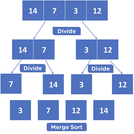
How MergeSort Works

MergeSort follows a divide and conquer approach:

1. It divides the input array into two halves recursively until each subarray contains only a single element.
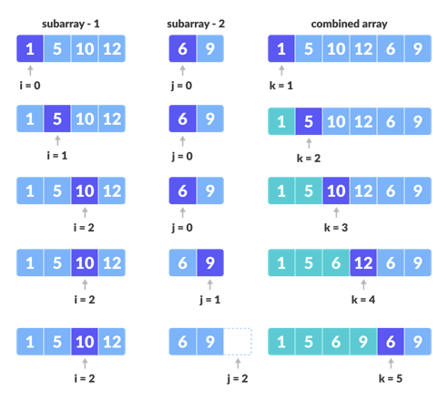
2. It then sorts and merges these subarrays by comparing elements pairwise and placing them in order.
3. The merging process continues recursively until all subarrays have been recombined into a fully sorted array.

This recursive splitting and merging make MergeSort efficient and predictable. Its worst-case time complexity is O(N log N), meaning the time required grows proportionally to N × log(N).

MergeSort is also a stable sorting algorithm, which means that two objects with equal keys maintain their relative order in the sorted output. As GeeksforGeeks defines stability:

“A sorting algorithm is said to be stable if two objects with equal keys appear in the same order in sorted output as they appear in the input data set.”
— GeeksforGeeks, 2011

An additional optimization sometimes applied to MergeSort involves replacing recursive calls with Insertion Sort for small arrays (typically of size ≤ 43). In these cases, Insertion Sort can outperform recursion due to its low overhead on small data sizes — though this optimization was not applied in this particular experiment.

---

Methodology

To compare the performance of MergeSort and QuickSort, we conducted an experiment measuring each algorithm’s runtime across arrays of increasing size.

Experimental Steps

1. Implementations:
   We used optimized Java implementations of both algorithms from GeeksforGeeks:

   • MergeSort Algorithm (2013)
   • QuickSort (2014)

2. Data Generation:
   A program was written to generate random integer arrays of varying lengths. The same data generator was used for both algorithms to ensure fairness.

3. Timing Measurement:
   Each algorithm’s runtime was recorded using Java’s System.nanoTime() function, calculating elapsed time by subtracting start time from end time.

4. Data Analysis:
   Each algorithm was tested ten times per array size, and the average runtime was recorded.
   Array sizes used in the tests included:
   0, 200, 400, 800, 1600, 3200, 6400.

Comparison Criteria

• Runtime performance (nanoseconds)
• Stability of sorting
• Growth rate of runtime with respect to N

By plotting average runtime versus array size, we could visually analyze efficiency patterns between MergeSort and QuickSort.

---

Variables

When running experiments of this nature, the following factors were carefully controlled:

• Input Array Size: Arrays ranged from small to large to observe performance across varying data scales.
• Data Distribution: Randomized values ensured uniform testing and minimized bias.
• Programming Language: Java was selected for consistency and class structure adherence.
• Environment:
  • Machine: MacBook Air
  • Processor: 1.6 GHz Dual-Core Intel Core i5
  • RAM: 16 GB (2133 MHz)
  • IDE: IntelliJ IDEA CE
• Number of Trials: Each test was repeated ten times, and the mean runtime was used to minimize anomalies.

---

Control Set

To maintain scientific validity, the following constants were upheld throughout all trials:

1. Identical Data Inputs for both algorithms.
2. Same Machine and Operating System for consistent performance measurement.
3. Same Compiler (IntelliJ IDEA CE) to ensure that no compilation-level optimizations influenced one algorithm differently from the other.
4. Repeated Trials to reduce statistical variance.

These control measures ensured that differences in runtime were due solely to algorithmic performance rather than external factors.

---

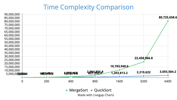
Results

The LazyArray generator was used to populate arrays with values ranging from 1 to 100,000.

Each array was sorted using both algorithms across sizes 0 → 6400, doubling the size in each iteration. The experiment revealed that QuickSort consistently outperformed MergeSort in every trial.

Array Size	QuickSort Runtime	MergeSort Runtime	Observation
200	Faster	Slower	Similar performance for small N
800	Faster	Slower	Gap widens noticeably
1600+	Dominant	Much slower	QuickSort ~150–215% faster

It was also observed that when data values were closely grouped, MergeSort approached QuickSort in performance — but QuickSort remained slightly faster overall.

---

Analysis

QuickSort outperformed MergeSort across all input sizes tested. While both algorithms share a theoretical O(N log N) time complexity, practical runtime differences arise due to recursion depth, memory allocation, and implementation specifics.

Property	QuickSort	MergeSort
Time Complexity (Average)	O(N log N)	O(N log N)
Time Complexity (Worst)	O(N²)	O(N log N)
Space Complexity	O(log N)	O(N)
Stability	Not Stable	Stable

At small input sizes (≤ 400 elements), both algorithms performed similarly. However, as N increased, QuickSort’s efficiency scaled better, while MergeSort’s runtime grew faster.

This can be attributed to:

• QuickSort’s in-place partitioning, which reduces memory usage.
• MergeSort’s recursive merging, which requires additional space.

That said, MergeSort remains the preferred choice when data stability is essential — such as when sorting records by secondary keys (e.g., sorting students by name after sorting by grade).

---

Conclusion

Our experiment set out to test the hypothesis that the runtime of MergeSort and QuickSort would both increase with input size, but at rates determined by their respective time complexities.

Key findings include:

• QuickSort consistently outperformed MergeSort for all tested array sizes.
• MergeSort’s performance remained predictable and stable, but slower due to higher space overhead.
• For large datasets, QuickSort proved more efficient, but MergeSort’s stability made it ideal for data requiring order preservation.

Algorithm Recommendations

Scenario	Recommended Algorithm	Rationale
Large dataset, stability not required	QuickSort	Fastest average runtime
Large dataset, stable output required	MergeSort	Stable and consistent
Small dataset	Insertion Sort	Minimal overhead
Specialized integer data	Radix Sort	O(M + N) efficiency

Ultimately, the choice of algorithm depends on the use case:

• QuickSort: Practical efficiency and lower space cost.
• MergeSort: Predictable performance and stability.
• HeapSort / RadixSort: Useful for specialized scenarios or constrained memory.

Both QuickSort and MergeSort exemplify the trade-offs between speed, stability, and space, forming the foundation of efficient sorting in computer science.

---

Bibliography

• Merge Sort Algorithm. (2013, March 15). GeeksforGeeks. https://www.geeksforgeeks.org/merge-sort/
• QuickSort vs MergeSort. (2018, September 28). GeeksforGeeks. https://www.geeksforgeeks.org/quick-sort-vs-merge-sort/
• Stable and Unstable Sorting Algorithms. (2011, January 20). GeeksforGeeks. https://www.geeksforgeeks.org/stable-and-unstable-sorting-algorithms/